Formula 1 To return the cell absolute reference. After INDEX returns a reference the formula resolves to.
How To Return Cell Address Instead Of Value In Excel Free Excel Tutorial
By wrapping INDEX in the CELL function we can get Excel to show us the address to the cell returned by INDEX.
Excel formula lookup return cell reference. In the result_vector argument you reference the column from which you want to return a value and your Lookup formula will fetch the value in the same position as the lookup value. If you want to return cell address instead of cell value in your formula how to do it. Just like any other reference Excel shows the value in the cell.
Advanced excel formulas can be used to lookup values or text in Excel and return the relative cell address. Select a blank cell here I select cell C3 enter the below formula into it and then press the Enter key. If you wish to get the number of the row holding the last value then use the ROW function to retrieve it.
Select the entire data range from the sheet 2 and write the formula as below VLOOKUPA1Sheet 2A2E4952FALSE - if you want to lookup Column B in Sheet2 VLOOKUPA1Sheet 2A2E4953FALSE - if you want to lookup Column C in Sheet2 VLOOKUPA1Sheet 2A2E4954FALSE - if you want to lookup Column D in Sheet2. Besides you can vlookup and get the adjacent cell value based on a cell reference. You could adjust the formula to create a hyperlink in the cell instead of just the address.
They dont act as a link to that cell. Match lookup_value range0 1 is to return the value where look_value is in range index range1 match_return col is to return the reference where match_return col is cell address index_return is to return the address of the lookup like C4. Many of us know the OFFSET function returns a reference to a range of cells but there are actually 8 Excel functions that return a reference to a range.
An INDEX function can be used to MATCH the lookup value in a range of cells. Find_text - the character or substring you want to find. With using cellindex and match this task could be done.
The VLOOKUP function in Excel performs a case-insensitive lookup. CTRL and CTRL look for cell precedents and dependents. Select a blank cell enter the below formula into it and then press the Enter key.
The function returns the value of an element in a table or an array selected by the row and column number indexes. Usually its supplied as a cell reference but you can also type the string directly in the formula. SWITCH new in Excel 2019 IF.
I could then use this ROW value in INDEX function. In the formulas the first A1A8 is the range where you look up for value and the second A1A8 is the range where you want to look up for the. VLOOKUPMAXA2A11 A2B11 2 FALSE Then the adjacent cell value of the largest weight in column A is populated in the selected cell.
Using INDEX function to return the value of a specified cell or array of cells. To return a reference to specified cells. IFS new in Excel 2019 INDIRECT.
Where sheet_name is a reference that contains the sheet name. After INDEX returns a reference the formula resolves to. You can then click on it and it will take you to the referenced cell.
For the example on this page the formula would be. INDEX function can be used in two ways INDEX reference and INDEX array. Each function has their pros and cons.
Use this if the first argument to INDEX is an array constant. Within_text - the text string to be searched within. How do I look up search for a value text in a table and return the cell reference.
For example if the lookup value of cell A2 is the number 4 then XLOOKUP will technically return A2 rather than 4 although youll only see 4. Lets take a look at them in turn. Search for the name John in B1F24 and if found return cell address say D6.
CELLaddress C8 returns C8. For example you have a range of data as below screenshot shown and you want to lookup product AA and return the relative cell absolute reference. INDEX array row_num.
INDIRECT B6 A1 Note this. Normally you can use INDEXMATCH function to lookup a value in a given range of cells and returns cell value. Select a cell and type AA into it here I type AA into cell A26.
Preferably Id like to find John and return the only the ROW number in my example 6. XLOOKUP returns a cell reference as the result rather than the value. Start_num - an optional argument that specifies from which character the search shall begin.
26 rows Returns a reference as text to a single cell in a worksheet. XLOOKUP Excel for Microsoft 365 only CHOOSE. Then type this formula CELLaddressINDEXA18A24MATCHA26A18A241 in the cell adjacent to cell A26 the cell you typed AA then press Shift Ctrl Enter keys.

Excel Formula Vlookup With Numbers And Text Exceljet

How To Use The Excel Lookup Function Exceljet
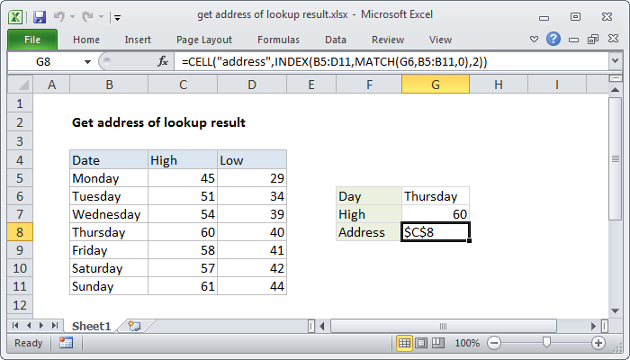
Excel Formula Get Address Of Lookup Result Exceljet

Vlookup Formula Syntax Explanation Amp Example Excel Formula Excel Tutorials Excel
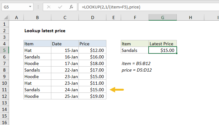
Excel Formula Lookup Latest Price Exceljet

Excel Formula Two Way Lookup With Vlookup Exceljet

How To Reference Cell In Another Excel Sheet Based On Cell Value Excel Microsoft Excel Formulas Excel Formula

Pin On Excel
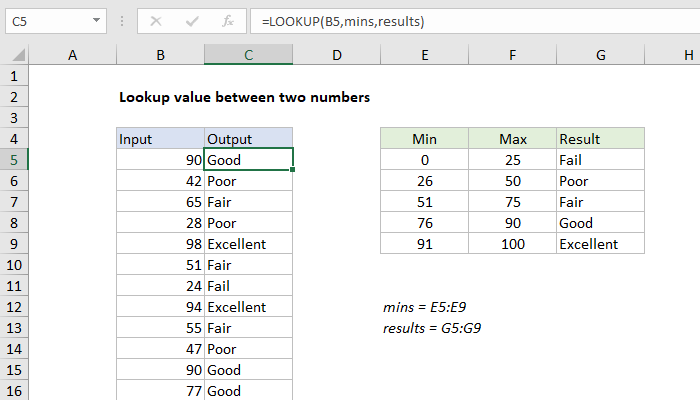
Excel Formula Lookup Value Between Two Numbers Exceljet

Tidak ada komentar:
Posting Komentar